You might also like our Microsoft Surface Pro 4 review, Windows 10 Review, and Microsoft Office 365 Vs Office 2013
How to make PivotTables in Excel: What is a PivotTable?
While it might sound like an avant-garde piece of designer furniture, a PivotTable is a data summary tool that can display information about large data sets in a customisable tabulated form. In simpler terms, it’s a clever trick that shows you what you want to know about stuff you already have in your spreadsheets. Say you have a large data set that includes a range of information about your business, and you want to know how much a certain project has cost or which salesperson has performed the best over a set period? To find this out you can either try dabbling with several formulas to generate these results, which could be complicated and time consuming, or you could create a PivotTable which does the hard work for you.
How to make a Pivot Table in Excel
Although the use of PivotTables can be complex, depending on just how deep you want to go, creating one is actually very easy. The first thing you need is a spreadsheet with data already present. Before you can start it’s important to ensure that there are no empty fields, columns or rows, as the PivotTable will assume that the data to be included ends there. When you have everything ready click on a cell in the data you want to summarise, it doesn’t matter which one, then go up to the ribbon menu and select Insert.
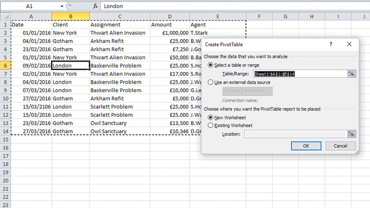
The first option on the left should be PivotTable. Click this and you’ll see that the data set has automatically been selected and a dialog box confirms the area that will be used for the PivotTable.
Below the Table/Range box you’ll see the options for creating the table in either a new worksheet or an existing one. For this walk-through we’ll select New. Click OK and the PivotTable will be created.
How to use a PivotTable
Initially it might look like things haven’t gone to plan, as the new worksheet is empty. This is meant to happen as one of the main advantages of PivotTables is that you can select which data fields you want to appear, and then change them as many times as you like to produce different reports.
In the right-hand corner of the screen you’ll see a list of fields you can choose to include. As you tick each box the PivotTable will begin to take shape in the main part of the screen. When you add fields the PivotTable will order them into related areas which show the breakdown of the information. In our example we wanted to know the individual costs of the various assignments that our agents had undertaken, so by selecting those fields we quickly knew the exact amounts of each project and how much each agent had been awarded.
That’s all well and good, but now we want to know how much revenue each client has generated. In a traditional spreadsheet this might take a while, but PivotTables work very quickly indeed to collate the information. There’s no need to create a new table, instead we untick the fields that we no longer need, and instead select the ones for the client, assignment, and amounts. Instantly the information is displayed in front of us. Very nice!
As we said earlier, PivotTables can be very powerful if you dig deeper into the various options available in the ribbon menu. These advanced features would take up an article all of their own, so we won’t be covering them today, but there is one area that it’s worth exploring briefly – Design.
How to change the layout of a PivotTable in Excel
At the top of the ribbon menu you’ll see the pink PivotTable Tools tab is highlighted. Directly underneath this are two more tabs – Options and Design – of which Options is currently selected. Click on Design and you’ll see a far simpler set of tools appear. In this menu you can shape how the information in the PivotTable is displayed. The first couple of options relate to whether you want Sub-Totals or Grand Totals in your table, but the one most people will want to start with is the Report Layout. Clicking this opens up a drop down menu with a few basic alternatives for the layout of the table. Again this is all dynamic, so you can click through each option without ruining your report, then return to your preferred design at the end.
Try spending a few minutes experimenting with the settings, until you’re happy with the look and feel of your report. There’s plenty more you can do with PivotTables, but at least with these initial steps you can start exploring how they can be put to work for your own needs. You never know, there might even be a large sticky donut in store at the next office meeting as people gaze upon your techno-wizardry with wonder. Well, you can dream can’t you? Martyn has been involved with tech ever since the arrival of his ZX Spectrum back in the early 80s. He covers iOS, Android, Windows and macOS, writing tutorials, buying guides and reviews for Macworld and its sister site Tech Advisor.